INTEGRATION OF BANANA MARKETS IN INDIA
M.S. Sadiq1, N. Karunakaran2 and I.P. Singh3
1Department of Agricultural Economics and Extension Technology, Federal University of Technology, Nigeria
2Department of Economics, EKNM Government College, India
3Department of Agricultural Economics, Swami Keshwanand Rajasthan Agricultural University, India
10.21917/ijms.2018.0104
Abstract
The present research used monthly time series data to investigate market integration of banana in India. Empirically, it was observed that the Law of One Price (LOP) was moderate in the horizontal integrated wholesale markets and robust in the retail markets. However, the LOP was found efficient in all the vertical integrated markets. Both from the horizontal and vertical dimension, Mumbai market was found to be the most efficient as they respond to price news in correcting their disequilibrium which arises from any of the shortrun equilibrium. In the event of any innovation (bad-news or goodnews), almost all the markets will be price follower in the banana market in India. Furthermore, banana trade is found to be very useful in all the selected markets as the volatility pattern is not explosive and Chennai market was the most efficient in price discovery. Lastly, future prices of banana in the selected markets will remain fair if well monitored in such a way that none of the participants in the marketing channel of banana will be better-off nay worse-off. Therefore, for the overall marketing efficiency, more resources should be allocated to those markets with a high degree of integration and market efficiency.
Keywords:Integration, Market, Banana, India
1. INTRODUCTION
A marketing chain which provides maximum benefits to all its participants along the chain is the marketing system that is well organized and efficient. The pre-requisites for an efficient marketing system are perfect market integration and perfect price transmission which if achieved will omit arbitrage which is not lucrative, thereby adjusting changes in price rapidly. Praveen and Inbasekar [5] reported that the present structure of the agricultural marketing system prevailing in India may not be conducive for improving marketing efficiency due to poor infrastructure and inadequate information dissemination which hinder healthy market integration of agricultural products. Therefore, to have a vivid understanding on the overall market performance, information on spatial market integration which will provide hints on operational efficiency, allocative efficiency, competitiveness and effectiveness of arbitrage along the chain of the transaction is necessary. Furthermore, the specifics on the market performance required for policy formulation and macroeconomic modelling can be given by the studies on market integration. Also, price signals transmitted by none, poorly and weakly integrated markets would deceive and mislead the producers’ in making decisions on marketing, thereby causing inefficiency in the movement of products. In view of the relevance of the information evolving out of studies on market integration, an effort was made to empirically discern the status of market integration of banana in India as the earlier study conducted by Praveen and Inbasekar [5] reported poor market integration of this fruit in India. The specific objectives conceived for this research were to examine the seasonal price and quantity of arrival index pattern of banana across the selected markets; to determine the extent and degree of market integration; to determine how prices were discovered in the individual markets and the causes of price volatility; and to forecast the future price of banana in all the selected markets.
2. RESEARCH METHODOLOGY
The study made use of monthly time series data spanning from January 2008 to January 2017 sourced from the National horticulture board of India. The data covered wholesale and retail market prices in Chennai, Ahmadabad, Mumbai and Hyderabad. Data analyses were performed using both descriptive and inferential statistics. In descending order, the first objective was achieved using descriptive statistics and centered 12 month moving average; the second objective by using Augmented Dickey Fuller test (ADF), Johansen co-integration test, restricted VAR model, distributed lag model-market index concentration, impulse response and Granger causality test; the third objective used seemingly unrelated regression (SUR) and GARCH models; and the last by the VECM model. The wholesale and retail markets in Chennai, Ahmadabad, Mumbai and Hyderabad were denoted by CWM and CRM, AWM and ARM, MWM and MRM, and HWM and HRM respectively.
2.1 EMPIRICAL MODEL
2.1.1 Percentage of Centered 12-Month Moving Average Method:
The ratio-to-moving average provides an index of seasonal and irregular components combined because
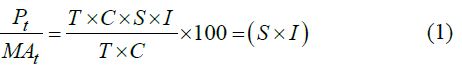
where, Pt is the price index observation at period t, MAt is moving average at period t, T is the trend component, C is the cyclical component, S is the seasonal component and I is irregular component.
Averaging this over years and adjustment through correction factor provides a better estimate of seasonal index.
where, K is correction factor and S is the sum.
2.1.2 Augmented Dickey Fuller Test:
Following Sadiq et al. [9], the autoregressive formulation of the ADF test with a trend term is given below:
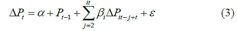
where, Pit is the price in market i at time t, α and ΔPit(Pit - Pt-1) is the intercept or trend term.
2.1.3 Johansen’s Co-Integration Test:
Following Johansen [3], multivariate formulation is specified below:
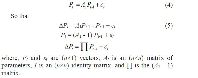
where, λi denotes the estimated values of the characteristic roots (Eigen-values) obtained from the estimated IT matrix, and T is the number of usable observations.
2.1.4 Granger Causality Test:
Following Granger [2], the model used to check whether market P1 Granger causes market P2 or vice-versa is given below,
2.1.5 Vector Error Correction Model (VECM):
The VECM explains the difference in yt and yt-1 (i.e. Δyt) and it is shown below [7] [8]:
It includes the lagged differences in both x and y, which have a more immediate impact on the value of Δγt.
2.1.6 Impulse Response Functions:
The GIRF in the case of an arbitrary current shock (δ) and history (ωt-1) [1] [6] is specified below:

2.1.7 Forecasting Accuracy:
For measuring the accuracy in fitted time series model, mean absolute prediction error (MAPE), relative mean square prediction error (RMSPE), relative mean absolute prediction error (RMAPE) [4], Theil’s U statistic and R2 were computed using the following formulae:

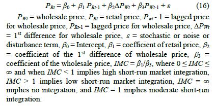
2.1.8 Index of Market Concentration (IMC):
The index of market concentration was used to measure price relationship between integrated markets, and the model is specified below:
2.1.9 GARCH Model:
The representation of the GARCH (p, q) is given as:
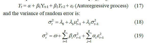
where, Yt is the price in the ith period of the ith market, p is the order of the GARCH term and q is the order of the ARCH term. The sum of ARCH and GARCH (α+β) gives the degree of persistence of volatility in the series. The closer is the sum to 1; the greater is the tendency of volatility to persist for a longer time. If the sum exceeds 1, it is indicative of an explosive series with a tendency to meander away from the mean value
2.1.10 Price Discovery using Seemingly Unrelated Regression (SUR):
The Garbade and Silber’s (GS) approach was used for estimating the efficiency of wholesale and retail markets in terms of price discovery. The basic structure of the model is given below:
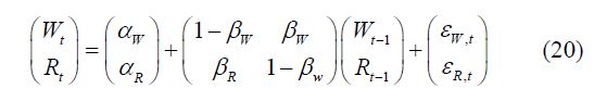
where, Wt is the monthly wholesale price at the ith period, Rt is the monthly retail price at the ith period, αW and αR reflect the constant secular trend in wholesale and retail markets respectively. The βW and βR reflect the influence of lagged price from one market on the current price in the other market. In the GS framework, the estimated equations are given as:
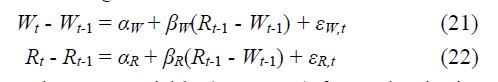
Here, the explanatory variable (Rt-1 - Wt-1) forms the ‘basis’ that is the difference between the wholesale and retail prices. The ‘basis’ variable should reflect the cost of capital from the trading date till expiry date and should contain a negative time trend, i.e.

The ‘basis’ was regressed for each time period, on a time variable (t-1), where t was the time to maturity of the retail market time period; and it was found that the estimated coefficient on time trend (βb) had turned negative, as expected. In the GS framework, Eq.(21) to Eq.(23) were estimated using ‘seemingly unrelated regression’ (SUR) model. If the estimated coefficient of βW is significant and βR is insignificant, the price discovery occurs only in the retail market. This would imply that the retail market is a pure satellite of the wholesale market and there is a convergence of wholesale and retail market prices because retail market prices move towards wholesale market prices. If βR is significant and βW is insignificant, price discovery occurs only in the wholesale market. If both βW and βR are significant, price discovery occurs in both the markets. If βR > βW, wholesale market dominates the retail market, and if βW > βR, retail market dominates the wholesale market. If both βW and βR are insignificant, then price discovery did not occur in either of the markets.
3. RESULTS AND DISCUSSION
3.1 SUMMARY STATISTICS OF MARKET PRICES AND QUANTITY OF ARRIVALS OF BANANA
A perusal of Table.1 revealed that the wholesale and retail markets with the highest and lowest prices were the vertically integrated market in Chennai and Ahmadabad respectively. In addition, the quantity of arrival was found to be highest in the former market and lowest in the later market. Also, observed was that the price of banana was stable in the Chennai market despite instability in its quantity of arrivals, and high in the rest of the selected markets.
The prices of banana in all the selected markets were asymmetrically distributed as their respective upper tail distributions were found to be thicker than their lower tail. However, the tails of the distributions were not thicker than the normal tail (kurtosis coefficient of < 3) for almost all the markets. Therefore, with the exception of CRM and the vertical integrated market in Hyderabad, none of the markets exhibited extreme price values as their respective kurtosis were small (Table.1).
3.2 SEASONAL PRICE INDEX PATTERN OF BANANA IN THE SELECTED MARKETS
A cursory review of the results of the seasonal price index pattern showed that in all the selected markets the price of banana was at its peak in the month of July when the quantity of arrivals was highest while the prices and their corresponding quantity of arrivals were found to be at the EBB during February (Table.2 and Fig.1 and Fig.2).
Therefore, the reason why prices were high when their corresponding quantities of arrivals were high may be attributed to efficiency in the marketing of banana in the country via minimization of the arbitrage tendencies of market participants.
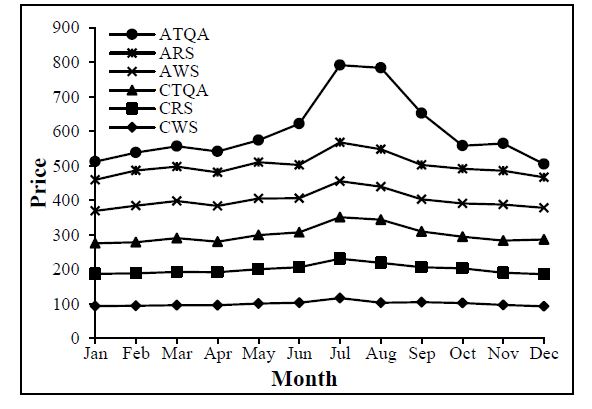
Fig.1. Seasonal price indices of Banana in Chennai and Ahmadabad
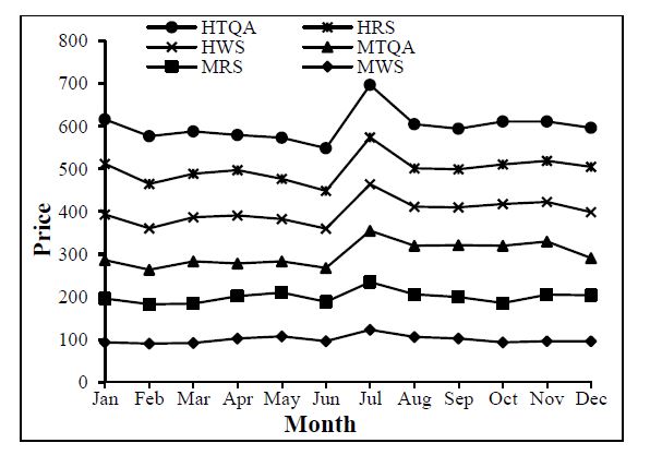
Fig.2. Seasonal price indices of Banana in Mumbai and Hyderabad
3.3 LAG SELECTION CRITERIA
Because of the sensitivity of the time series to lag length, the chosen lag for truncation that will make the model parsimoniously and ensure that the error term is Gaussian white noise is lag 1 as unanimously agreed by all the selection criteria viz. Akaike information criterion (AIC), Hannan-Quinn information criterion (HIC) and Bayesian information criterion (BIC) as indicated by their respective asterisk sign (Table.3).
3.4 UNIT ROOT TEST
The results of the ADF unit root test showed both the wholesale and retail price series not to be stationary at their respective levels (estimated tau-stats greater than t-critical values at 5% degree of freedom) but were found to be stationary at their respective first difference (estimated tau-stats less than t-critical values at 5% probability level). Also, the KPSS unit root test rejected the null hypothesis of absence of unit root in favour of alternative hypothesis of presence of unit root at level for all the variable price series (t-stats greater than the t-critical value at 5% risk level) but after the first difference the test accepted the null hypothesis of absence of random walk in the residuals of each of the variable price series against their alternative hypothesis of non-stationary (t-stats less than the t-critical value at 5% risk level). Furthermore, the ADF-GLS unit root test applied at the level to all the price series indicated non-stationary of the price series but after first difference they became stationary, thus, implying that the unit root test results generated by the conventional or traditional unit root techniques were robust (Table.4). Therefore, since both the wholesale and retail price series satisfied the pre-requisite for the application of cointegration test as their respective variable series are integrated of order one [I(1)].
3.5 THE LAW OF ONE PRICE (LOP)
The multivariate horizontal-wise results for the wholesale and retail markets showed the ranks of co-integration to be one and three respectively. The implication is that the market prices in both markets move together in the long-run but the extent of the horizontal integration was moderate in the wholesale market as the law of one price (LOP) hold in only two markets (CWM and AWM) out of the four selected markets which may be attributed to autarkic activities of the market middlemen while the extent of the horizontal integration was good in the retail markets as the LOP was found to hold in all the selected markets (CRM, ARM and MRM) which may be attributed to free flow of quantity of arrival and perfect flow of price information (Table.5). It is worth to note that the max-test is more powerful than the trace test.
The presence of two common stochastic trends (hence two independent markets) and one common stochastic trend for wholesale and retail markets respectively implies the presence of pair-wise cointegation of prices. For the horizontal pair-wise wholesale market co-integration results, with the exception of the market pairs viz. CWM-AWM and AWM-MWM which move together in the long-run, all the remaining market pairs have no long-run association. In the case of the retail market in the pair at the same level, with the exception of CRM-HRM, all the markets shared the same or have one stochastic trend, an indication that price differential between the markets in the pair are equal to the cost of transfer of banana despite their geographical spatiality’s (Table.6). Furthermore, the vertical pair-wise market co-integration results showed that all the wholesale markets to be integrated with their respective adjunct retail markets an indication of vertical market integration as the price differentials between the wholesale markets and their respective retail markets were equal to the cost of transfer of banana fruit. This outcome showed efficiency in the mechanism of banana marketing across the marketing channel which is due to a perfect flow of information, adequate market infrastructure and adequate quantity of arrivals (Table.6).
3.6 THE DEGREE OF MARKET INTEGRATION
The multivariate horizontal-wise VECM results for wholesale and retail markets showed that markets viz. AWM, MWM and HWM; and, all the retail markets respectively established long-run equilibrium irrespective of any short-run shock that emanated from any of the markets as evidenced by the significance of their respective attractor coefficients (Table.7). With the exception of AWM and MRM which diverge from the equilibrium, all the other markets converge to the equilibrium as indicated by the signs of their respective attractor coefficients (ECTt-1). Therefore, wholesale markets AWM, MWM and HWM; and retail markets CRM, ARM, MRM and HRM absorbed 5.9%, 5.7% and 11.93%; and, 12.46%, 14.53%, 10.56% and 22.30% shocks respectively to bring about price equilibrium in the long-run. The time required for information flow in the wholesale and retail markets were very fast as it will take approximately 1.77 days, 1.71 days and 3 days in AWM, MWM, and HWM respectively; and, 3.74 days, 4.36 days, 3.17 days and 6.70 days in CRM, ARM, MRM and HRM respectively, as indicated by their respective magnitude coefficients. Therefore, the MWM and MRM among the wholesale and retail markets were the most efficient in terms of reaction to the news on price.
The autocorrelation and arch effects exonerate the residuals of both the wholesale and retail markets VECM from the problem of serial correlation and arch effects as indicated by their respective Ljung-Box Q-stats and LM test-stats which were not different from zero at 10% degree of freedom. However, the test of normality showed that their residuals were not normally distributed as evidenced by their respective Chi2 tests which were different from zero at 10% probability level. Though non-normality in the distribution of residuals is not considered a serious problem as in most cases data are not naturally distributed (Table.8).
The results of the vertically integrated markets showed that only the vertical integrated market in Mumbai reciprocate in terms of reaction to news on price as evidenced by the significance of the attractor coefficients of the wholesale and its adjunct retail market (Table.8). Hence, the wholesale market is more efficient than the retail market in responding to price news as it will take less than an hour in a month in the former to re-established long-run price equilibrium when compared to the later which required almost an hour in a month to correct its disequilibria. For the markets in Chennai; and, Ahmadabad and Hyderabad the speed of price flow was unidirectional as only their respective retail and wholesale markets respectively were found to correct their deviation from the equilibrium due to any available price news shocks from the short-run equilibrium. For the markets which established long-run equilibrium, markets viz. AWM, MWM, HWM converges to their respective equilibrium while CRM diverges from its respective equilibrium. The autocorrelation and arch effect test for all the bivariate vertically integrated VECM exonerated their residuals from the problem of serial correlation and auto-covariance as evidenced by their respective Ljung-Box Q-stats and Lagrange multiplier test stats which were not different from zero at 10% probability level. However, their respective residuals failed the test of normality, but non-normality is not considered a serious problem as data in most cases are not normally distributed (Table.9).
3.7 GRANGER CAUSALITY TEST
The results of the direction of price information flow for the horizontal and retail market pair-wise showed that market pair viz. AWM-MWM; MWM-CWM, MWM-HWM, HWM-CWM; and, CWM-AWM had bidirectional causality, unidirectional causality and no causal relation respectively; while, CRS-ARS; MRS-ARS, HRS-CRS and HRS-ARS; and, CRS-MRS and MRS-HRS had bidirectional causality, unidirectional causality and no causality respectively (Table.10). The bidirectional causality implies that the market pair reciprocates price transmission as there is feed forward and feed backward in price formation. In the case of unidirectional causality, only one market in the pair dominates in price formation as its price effect is transmitted to later whereas the effect of price change in the later in the pair is not felt by the former. For the market pair with non-causal relation, it implies that the markets in the pair are independent of each other in price formation as none of the markets in the pair determines the price in each other market. In this case, external influence plays the crucial role in price formation in markets with no Granger causality effect.
Therefore, it can be inferred that the MWM market is the most efficient in the banana market as it takes the lead in price ruling as evidenced by its effect on almost all the selected markets. This might be attributed to adequate quantity of arrivals in the market, adequate marketing infrastructure and minimal market racketeering by the middlemen. However, the extent of efficiency in price formation between the retail markets was robust as the market with leading price ruling effect (HRS) has influence on two markets CRS and ARS, and the ARS has synergy in price formation with CRS.
For the vertically integrated markets the Granger causality results showed unidirectional causality to exist between market pairs: CRM-CWM AWM-ARM and HRM-HWM; and non-causality between the market pair: MWM-MRM (Table.11). This implies that the retail markets in Chennai and Hyderabad had ruling effect in the formation of prices in their respective wholesale markets with no effect of prices in turn from their respective wholesale markets. In addition, it means that price at the receiving end i.e. price paid by the consumers in these destination determines the direction of price in the wholesale markets. However, the opposite was the case in Ahmadabad as it was a feed-forward situation and not feed-backward situation. Therefore, the market integration direction in Chennai and Hyderabad were backward integration while that of the Ahmadabad was forward integration.
It is worth to note that a situation of strong endogeneity was not observed between any of the vertical integrated, an indication that exogenous factors play a crucial role in the formation of prices across market channels.
3.8 EFFECT OF INNOVATION (BAD-NEWS OR GOOD-NEWS) ON MARKET PRICES
Depicted graphically in Fig.3, Fig.4, Fig.5, Fig.6, Fig.7 and Fig.8 are how and to what extent innovation be it good-news or bad-news local to the prices of one of the banana markets affects the current and as well as the future prices in all the integrated markets over a period of twelve months. The Fig.3 for the wholesale in multivariate horizontal dimension showed that a shock local to CWM will have a permanent effect on AWM and transitory effects on itself and the remaining wholesale markets. An orthogonalized shock originating from AWM will not die-off in markets CWM, MWM and HWM; but will die-off in its own market within a short period of time. In addition, results showed that invention of bad-news in both MWM and HWM will have a lasting effect on only AWM market and transitory effects on the remaining markets inclusive its own market. Therefore, it can be inferred that with the exception of AWM all the remaining wholesale markets are relatively price followers and do not play role in the national banana market of the country as the extent of shock from these markets on other markets are less. The Fig.4 of the multivariate retail market horizontal-wise dimension depicted ARM and MRM to be the major price determinants in the retail market as shocks emanating from these markets are to a large extent transmitted to all the selected banana retail market in India. In addition, it showed that these aforementioned retail markets are the major game changer in the price of banana among the selected retail markets in India. In the case of the vertical-wise impulse response, unlike wholesale and retail markets in Chennai and Hyderabad whose shocks are transmitted to each other, the wholesale market in Ahmadabad is a price follower while both markets in Mumbai are independent of each other in terms of price shocks emanating from each channel in the marketing of banana (Fig.5 to Fig.8).
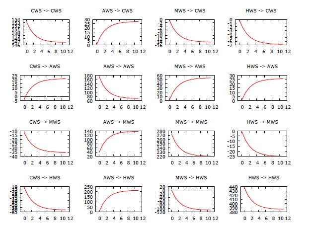
Fig.3. Horizontal-wise impulse response of wholesale markets
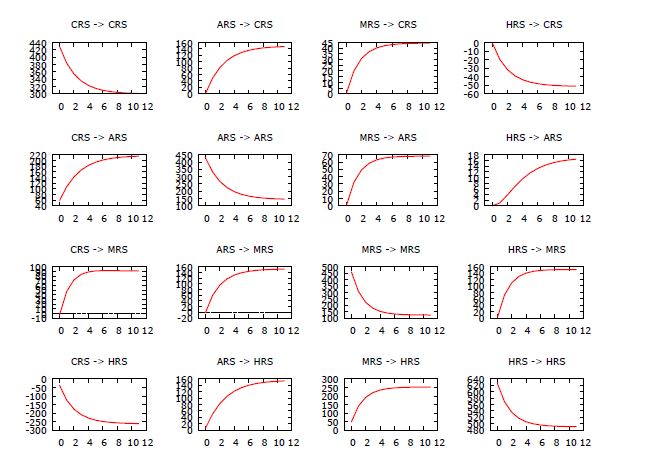
Fig.4. Horizontal-wise impulse response of retail markets
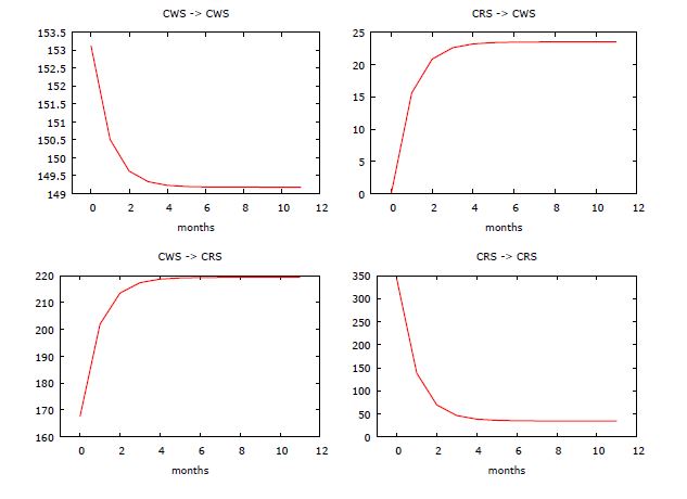
Fig.5. Vertical-wise impulse response in Chennai market
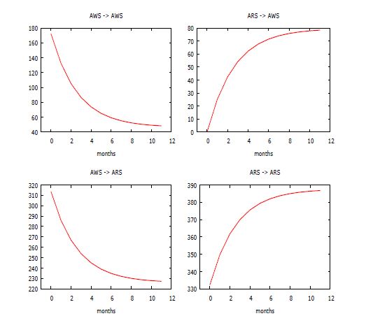
Fig.6. Vertical-wise impulse response in Ahmadabad market
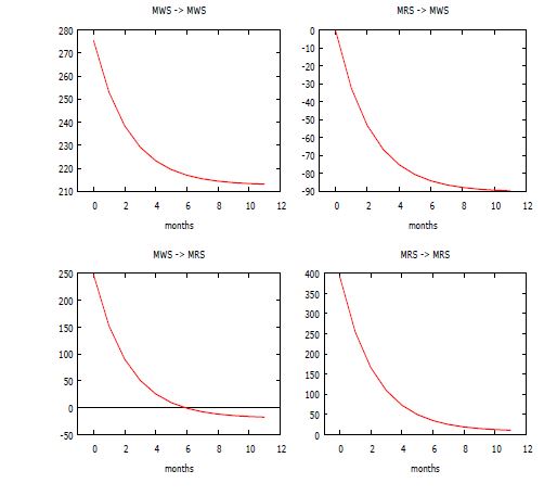
Fig.7. Vertical-wise impulse response in Mumbai market
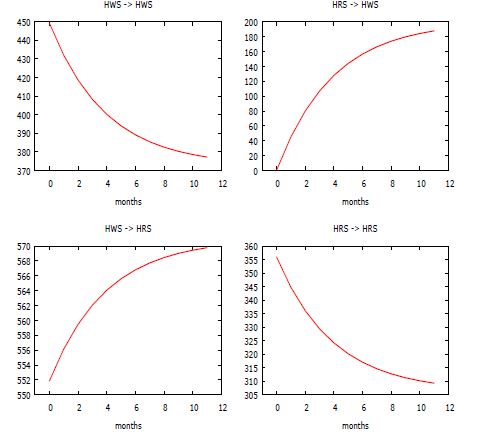
Fig.8. Vertical-wise impulse response in Hyderabad market
3.9 EXTENT OF MARKET CONCENTRATION
The results of market concentration index for backward vertical integration markets showed market pairs viz. CWMCRM; and, AWM-ARM, MWM-MRM and HWM-HRM have high and low short-run market integration as indicated by their respective concentration indexes which were less and greater than unity respectively (Table.8). Therefore, it implies that changes in the CRM retail market prices caused immediate changes in its wholesale market, while price changes in ARM, MRM and HRM do not cause immediate changes in the prices of banana obtained in their respective wholesale markets.
The diagnostic test results viz. autocorrelation, homoscedasticity,
arch effect, structural stability test; and multicollinearity
exonerated the results from the problem of serial
correlation, heteroscedasticity, arch effects, covariance and model
misspecification as evidenced by their respective t-statistics
which were not different from zero at 10% degree of freedom of
the model; and, the variables variance inflation factors which
were less than 10.00. However, the tests of normality for residual of each of the backward vertical integrated markets were found to be positively skewed as indicated by their respective t-statistics which were different from zero at 10% risk level. Though, non-normality in the distribution of residuals is not considered a serious challenge as data in most cases are not normally skewed. Therefore, it can be inferred that the distributed lag model is the best fit for the specified equation.
3.10 PRICE DISCOVERY IN BANANA MARKET
The results of annual price discovery in each of the markets for the period of ten years are presented in Table.9 and it showed that all the ten periods in Chennai markets were efficient in the discovery of price with the retail market been a pure satellite of its wholesale market. In Ahmedabad market, seven out of ten periods play a significant role in price discovery and its wholesale market dominated in the process of price discovery with its retail market been its pure satellite. Eight periods were found to be very efficient in the discovery of price in Mumbai market with the wholesale market dominating in the process of price discovery and the retail market been a pure satellite of the wholesale market. For the eight useful periods that were efficient in the process of price discovery in Hyderabad market, it was observed that price discovery occurred in its wholesale market. This implies that the retail market located in Hyderabad is a pure satellite of the wholesale market and there is a convergence of the wholesale and retail prices because the retail prices move towards the wholesale prices. However, it is worth to note that the situation of price discovery in both markets or non-discovery in the vertically integrated market was not observed for the ten periods cross-examined in the process of price discovery.
3.11 PRICE VOLATILITY
The mean equation for each of the wholesale markets certified the pre-condition for the application of ARCH and GARCH models as their respective residuals exhibited clustering volatility (graph not presented) and have arch effects present in them as evidenced by their respective Langrage multiplier test statistics which were different from zero at 10% degree of freedom (Table.10). The results of volatility in the forward vertical integrated markets presented in Table.10 showed that volatility in the current banana prices in Chennai and Ahmedabad markets will depend on external shocks which is their respective retail markets; and, information on the preceding month price volatility and preceding month price volatility. The volatility in the current banana prices in Mumbai and Hyderabad markets will rely on their external shocks and respective information of price volatility in the preceding month. Therefore, external shocks plays crucial role in the current volatility that will be experienced in all the selected banana markets as evidenced by the significance of their respective exogenous coefficients while the role of family shock was total in CWM and AWM; and partial in MWM and HWM as evidenced by the significance of both ARCH and GARCH terms; and, ARCH term respectively. Each wholesale market had its estimated sum of α+β to be close to 1, indicating high volatility in the spot prices of banana in the selected wholesale markets which will persist for long. Therefore, since none of the price series will likely meander away from the mean as indicated by the non-existence of explosive volatility pattern in the price series (α + β is not greater than 1 for each of the wholesale markets), it can be inferred that banana trade is very useful in the selected banana markets in India. The reason for volatility persistence in the prices of banana could be due to seasonality which affects the quantity of arrivals in the selected major banana producing regions in the country. The autocorrelation test showed that the residuals of the model are not serial correlated as indicated by their respective Q-stats which were not different from zero at 10% probability level. However, the residuals were found not to be normally distributed except for MWM as indicated by their Chi2 values which were different from zero at 10% degree of freedom. Though, this should neither put a question mark on the validity of the GARCH model nor be a source of concern as Sadiq et al. [9] reported that in most cases data are not normally distributed. In addition, the LR chi2 test for the GARCH model showed that the ARCH and GARCH terms are different from zero as indicated by their respective Chi2 values which were significant at 10% probability level. Therefore, the GARCH (1,1) model is the best fit for the specified volatility equations.
3.12 PRICE FORECAST OF BANANA IN THE SELECTED MARKETS
3.12.1 Diagnostic Checking and Validation:
The VECM was found to be appropriate in forecasting the price series of the selected markets as indicated by the multivariate horizontal VECMs diagnostic test results which exonerated their respective residuals from the problem of autocorrelation and arch effect as shown by the Ljung-Box Q-stats and Langrage multiplier tests respectively which were not different from zero at 10% risk level (Table.9). Therefore, the absence of random error means that the market prices are predictable, which is good for policy making, consumer decision and consumption pattern.
3.12.2 Validation (ex-post Prediction Power):
Though price movement predictability is in contrast to the efficient marketing theory as the theory posit that for a market to operate efficiently, prices should be unpredictable in that if they are stationary and predictable they will attract investors and their active participation will ultimately result to the cancellation of the prediction. However, this deductive (theory) idea has little empirical extent as inductive (facts) knowledge showed that prediction of prices is very important in measuring market efficiency except that the prediction should not be too long. One-step-ahead forecast of the prices along with their corresponding standard errors using naïve approach for the period September 2017 to January 2018 (total 5 data points) in respect of the VECM fitted models were computed to determine the predictive power of the estimated equation (Table.15). This was done to examine how closely they could track the path of the actual observation.
The price forecasting ability of the wholesale and retail market prices was measured using the mean absolute prediction error (MAPE), root mean square error (RMSE), Theil’s inequality coefficient (U) and the relative mean absolute prediction error (RMAPE) (Table.16). The results indicated the accuracy of the price forecasted as shown by their respective market RMAPE and U which were less than 10% and equal to 1 respectively. Therefore, these relatively low values indicated the consistency of the forecasted prices with the actual prices.
3.12.3 Forecasting:
One step ahead out of sample forecast for banana prices (Rupees per quintal) for the wholesale and retail markets from February 2018 to January 2019 were computed. This short span prediction was made in order not to affect market efficiency as long prediction will attract investors which will lead to the breakdown of the forecasted price (Table.17 and Fig.9 and Fig.10).

Fig.9(a). Wholesale prices of banana in CWM

Fig.9(b). Wholesale prices of banana in AWM
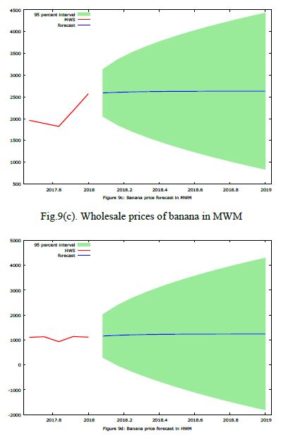
Fig.9(c). Wholesale prices of banana in MWM

Fig.9(d). Wholesale prices of banana in HWM
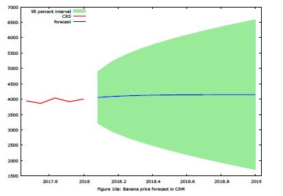
Fig.10(a). Retail prices of banana in CRM

Fig.10(b). Retail prices of banana in ARM
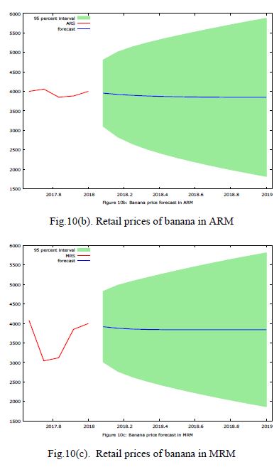
Fig.10(c). Retail prices of banana in MRM
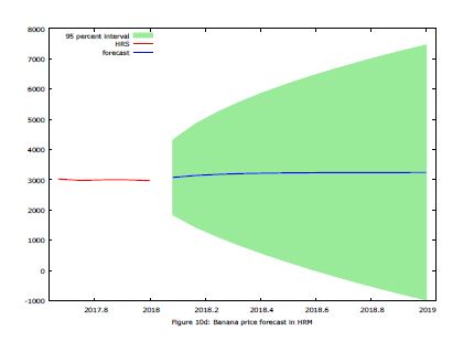
Fig.10(d). Retail prices of banana in HRM
It was observed that CWM, MWM and HWM markets will witness a very slight increase in their respective prices till the early month of their last quarter and thereafter will flatten out after a gentle very slight fall in the prices. The price of the banana in AWM will be oscillating throughout the month range from February to September 2018, remain flat till October and thereafter a slight fall which will flatten-out till January 2019. In the case of the retail markets, the retail prices of CRM, ARM and HRM will exhibit an oscillating (upward-downward swing) trend throughout the forecasted periods whereas the retail prices in MRM will witness an oscillating behaviour till July 2018, then a slight decline which will flatten-out till November 2018 and thereafter a slight increase which will maintain a flat trend till January 2019. The rate of price instability across all the markets will be mild as observed from their respective standard error values (not reported). Therefore, the technical and pricing efficiencies of banana should be monitored in such a way that neither the farmer nor the consumer nay the middlemen will be better-off nor worse-off in the marketing channel of banana in India.
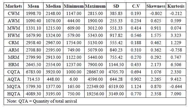
Table.1. Summary statistics of market prices and quantity of arrivals
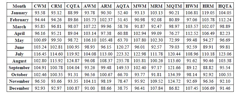
Table.2. Seasonal indices of monthly prices of Banana in selected markets (2011-2017)

Table.3. Lag Selection Criteria
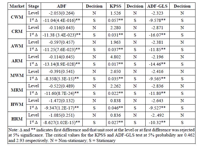
Table.4. Unit Root Test Results
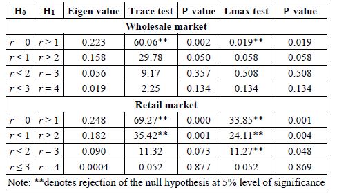
Table.5. Multivariate Horizontal-wise Cointegration Results
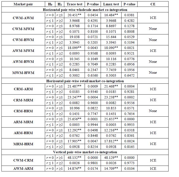
Table.6. Pair-wise Market Co-Integration
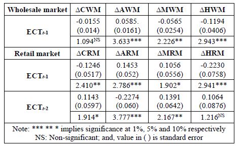
Table.7. Multivariate Horizontal VECM Results
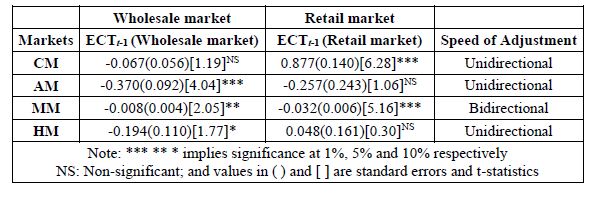
Table.8. Bivariate Vertical-wise VECM
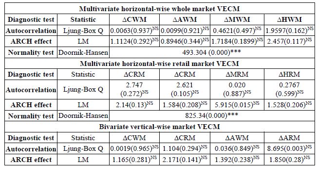
Table.9. VECM Diagnostic test results
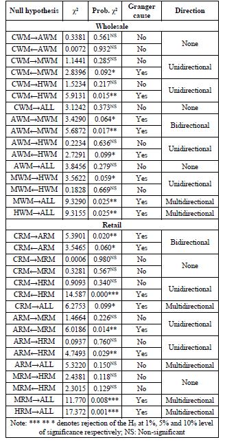
Table.10. Horizontal pair-wise Granger causality test results
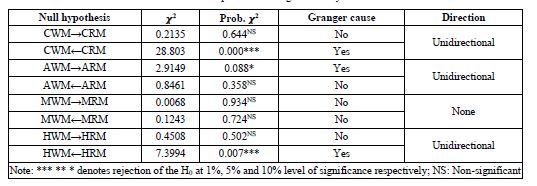
Table.11. Vertical pair-wise Granger causality test results
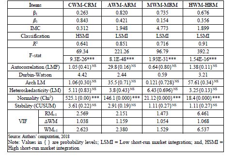
Table.12. Indices of market concentration
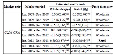
Table.13. Price discovery of pair-wise vertical integrated markets
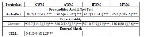
Table.14. Price volatility of banana in the wholesale markets
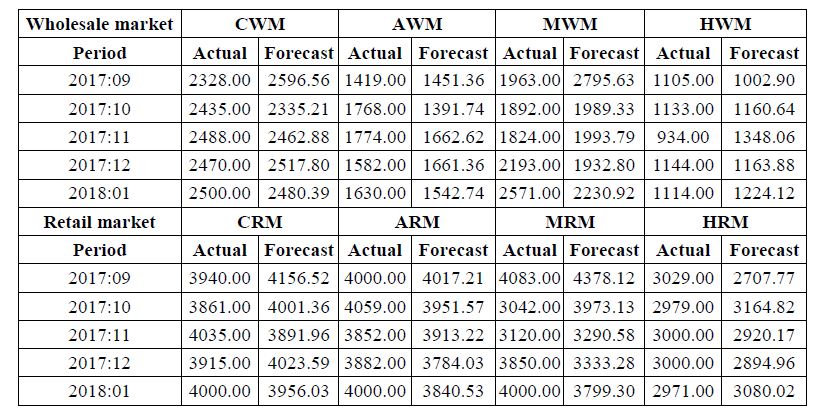
Table.15. One step ahead forecast of prices
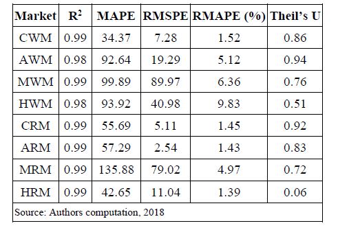
Table.16. Validation of models
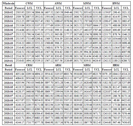
Table.17. Out of sample forecast of banana prices in selected wholesale and retail markets (Rupees per quintal)
4. CONCLUSION AND RECOMMENDATIONS
Findings from this study showed the extent of horizontal market integration to be moderate for the wholesale markets and good for the retail markets as the LOP was weak in the former and very effective and efficient in the later market. In addition, the degree of market integration was found to be most efficient in Mumbai market as the markets at different marketing stages react very fast to price news in correcting their respective price deviation from the equilibrium. Also, the degree of vertical integration showed the Mumbai market to be efficient as both markets reciprocate to a reaction in price news. It can be concluded that banana marketing is very useful in all the selected banana markets in India as none of the price series exhibited explosive volatility pattern. Also, concluded was that Chennai market was the most efficient in the process of price discovery as prices were discovered in all the ten periods. Lastly, the future prices of banana in all the selected markets will be mild in such a way that neither the wholesalers nor the retailers nay the producers or consumers will be worse-off nor better-off in banana marketing. Therefore, in order to enhance the overall efficiency of the marketing function and minimization of distortion in the marketing of banana, more resources should be allocated to those markets with a high degree of integration and market efficiency.
REFERENCES
[1] F.A. Beag and N. Singla, “Co Integration, Causality and Impulse Response Analysis in Major Apple markets of India”, Agricultural Economics Research Review, Vol. 27, No. 2, pp. 289-298, 2014.
[2] C.W.J. Granger, “Investigating Causal Relations by Econometric Models and Cross-Spectral Methods”, Econometrica: Journal of the Econometric Society, Vol. 37, No. 1, pp. 424-438, 1969.
[3] S. Johansen, “Statistical Analysis of Co-Integration Vectors”, Journal of Economic Dynamics and Control, Vol. 12, No. 2-3, pp. 231-254, 1988.
[4] R.K. Paul, “Forecasting Wholesale Price of Pigeon Pea using Long Memory Time-Series Models”, Agricultural Economics Research Review, Vol. 27, No. 2, pp. 167-176, 2014.
[5] K.V. Praveen and K. Inbasekar, “Integration of Agricultural Commodity Markets in India”, International Journal of Social Sciences, Vol. 4, No. 1, pp. 51-56, 2015.
[6] M.M. Rahman and Shahbaz, “Do Imports and Foreign Capital Inflows Lead Economic Growth? Cointegration and Causality Analysis in Pakistan”, South Asia Economic Journal, Vol. 14, No. 1, pp. 59-81, 2013.
[7] M.S. Sadiq et al., “Extent, Pattern and Degree of Integration among Some selected Cocoa Markets in West Africa: An Innovative Information Delivery System”, Journal of Progressive Agriculture, Vol. 7, No. 2, pp. 22-39, 2016.
[8] M.S. Sadiq et al, “Price Transmission, Volatility and Discovery of Gram in some Selected Markets in Rajasthan State, India”, International Journal of Environment, Agriculture and Biotechnology, Vol. 1, No. 1, pp. 74-89, 2016.
[9] M.S. Sadiq et al, “Volatility and Price Discovery of Palm Oil in International Markets under Different Trade Regime”, Journal of Agricultural Economics, Environment and Social Sciences, Vol. 3, No. 1, pp. 33-50, 2017.