ICTACT Journal on Management Studies
Volume 2, Issue 2 - May 2016
MANAGING THE ECONOMIC REPLACEMENT OF AN OPERATIONAL VEHICLES: A HEURISTIC DECISION MODEL
Mohammed Shurrab1, Ghaleb Abbasi2, Marwan Al-Taweel3
1Department of Mechanical Engineering, Kyushu University, Japan
2Department of Industrial Engineering, University of Jordan, Jordan
3Directorate of Maintenance, The Royal Jordanian Air Force, Jordan
DOI:
10.21917/ijms.2016.0038
Abstract :
A heuristic decision model for the replacement of an operational vehicle was developed. The proposed model is based on analysingan economic measures incorporating the most important factors such as: operation and maintenance costs, salvage values, depreciation, cost of capital, and most importantly, unavailability costs to reflect the hidden off-road vehicle costs. Parameterization of life-cycle costs, classification of existing vehicles, and vehicle priority factors were demonstrated in a case study for the Royal Air Force vehicles fleet. It is worth mentioning that the proposed heuristic is a beneficial tool in replacement decision and in making trade-off analysis among viable replacement strategies.
Keywords:
Replacement Analysis, Operational Vehicles, Economic Analysis, Trade-off Analysis
1. INTRODUCTION
The decision to keep or replace a vehicle involves the evaluation of costs and benefits for each proposed alternative [1]. The principles of engineering economy are utilized to analyse alternative uses of financial resources. The evaluation should depend on applying cost data analysis concerning the most important economic factors. Such factors are related to equipment usage as operation and maintenance costs, salvage values, depreciation, work delivered (i.e. working hours or vehicle distance), the cost of capital, tax credits (if exists) [2], [3]. The most important decision is the choice between keeping and replacing the operational vehicle during the remaining anticipated life. The existing vehicle operating in service (under study) is called the defender while, the challenger is the perspective of a replacement vehicle proposed as an alternative of the existing one, considered as the representative of the Defender vehicle group class [4].
Factors other than economy often enter into vehicle replacement analysis. Availability is defined as the probability that the system (such as a vehicle) is operating at any random time [5], [6]. This can be accomplished when management guarantees that the service of a certain vehicle can be provided and performed with less down-time and high dependability. In addition to avoid wasted time in the workshop due to long diagnosis time and difficult troubleshooting, shortages of workable spares, and long duration of maintenance and repair malfunctions. Here, it’s mandatory to express the value of unavailability and unserviceability by weighting its measured cost. Thus, a new additional concept of recurring cost will be introduced through the analysis to ensure that vehicle fleet will meet both operational reliability requirements and economic considerations.
Several researchers have discussed the replacement problem. Drinkwater and Hasting [7] used repair limits that provide an economic replacement strategy based on repair limit equation or particular frequency distribution for repair cost. Also, Thompson [8] used mathematical model for optimum replacement to minimize total expected cost of providing operating and maintenance costs. R.N. Wadhawan and F.G. Miller [9] proposed an appropriate methodology to obtain reasonably accurate forecasts of fleet vehicle replacement. Matsuo [10] presented a modified approach to the replacement of an existing asset. A procedure was developed to replace an existing asset, which has an arbitrary marginal cost. The procedure provides a set of alternative strategies for the owner of the asset, which enables the owner to make trade-offs between viable strategies. Love and Guo [11] presented a Markov approach to repair limit analysis. The repair limit policies were structured by dividing the life of the vehicle into a number of ages. Each age was treated as a state, associated with each state was a failure pattern modelled as either a homogenous or a non-homogenous Poisson process. Pedraza‐Martinez and Van Wassenhove [12] provided a study onvehicle replacement within the International Committee of the Red Cross. They showed empirically that significant savings can be made by studying humanitarian fleet management in developing countries. However, most of the previous studies [13]-[15] discussed the equipment and vehicle replacement problem taking into account future changes in capacity requirements, conditions of fleet work, maintenance and repair policy, vehicles ages, type and functions, and others.
The main goal of this research is to propose and develop a simple, direct model to assist in defining and evaluating available alternatives based on both economic and availability approaches to provide a tool to aid in the decision making process. A case study was also demonstrated the developed heuristic.
2. LIFE-CYCLE COSTS
Life-cycle cost is the sum of all expenditures associated with a vehicle during its entire service life [16], [17]. It consists of first cost, operation and maintenance costs, and salvage value [18]. A cash flow profile of both the defender and challenger is constructed based on historical data of existing vehicles and historical records of vehicle procurement. Knowledge of vehicle-use pattern and service vehicle circumstances in an organization dictates vehicle-cost pattern. Estimates of the functionally useful physical life of an item of equipment may be obtained from manufacturers and suppliers. Alternatively, if a company repeatedly buys a particular item of equipment and keeps accurate maintenance records, these records may be used to obtain an estimate of the functional life of item [19]. New cost estimate will be determined based on historical data.
The defender’s cash flow during its remaining service life will depend on predictions and estimations of the anticipated remaining service life, present resale market value, vehicle annual fixed cost, vehicle annual variable cost, anticipated salvage value, and resale values of vehicle during years of service. Once the existing vehicle salvage value is determined, its resale values during the remaining years of service can be estimated based on depreciation values since age of the vehicle is the most important factor in determining trade-in value. Also, total annual cost (TAC) of the defender during its anticipated remaining life will be evaluated using forecasting techniques based on historical data. The evaluation of challenger, as the perspective of future available replacement vehicle, life-cycle cost will be estimated as a main part in the model analysis, to develop the necessary estimation of challenger equivalent uniform annual cost (EUACch). For the purpose of applying the analysis to perform the heuristic, the following assumptions and criteria are valid:
- 1. The existing vehicle and the available replacement vehicle anticipated useful life should be assumed. The existing vehicle and the available replacement vehicle should have the same group class.
- 2. Inflation effect is neglected.
- 3. The challenger is replaced by another vehicle every time of period indefinitely. This time period is the economic life of minimum cost of challenger.
- 4. Study period of the analysis is equal to the anticipated remaining service life of the Defender [10].
3. PROPOSED METHODOLOGY
The following methodology is used to formulate the heuristic:
- 1. Construct the existing vehicle life-cycle costs for its anticipated remaining service life. This leads to the estimation of total marginal costs for year j for the defender(TMCj).
- 2. Construct the available replacement vehicle life-cycle costs during its anticipated service life. Estimate the defender group class cost profile as a challenger cost profile, i.e. (EUACch).
- 3. Present unavailability measure based on new annual expenses that will be included in the analysis when defining and evaluating vehicle unavailability cost (VUC) for both defender and challenger.
- 4. EUACch and TMCj are used to calculate future worth cost advantage (FWCAj) of replacement strategies that leads to finding a set of alternative strategies of replacement along with the best one.
Next, the above steps are discussed.
3.1 DEFENDER’S VEHICLE LIFE-CYCLE COSTS
The following input data should be known based on assumptions and certain considerations, in order to evaluate the defender’s life-cycle costs:
- 1. Age of defender vehicle = g.
- 2. Defender starting service year.
- 3. Defender group class.
- 4. Anticipated remaining service life (n), where, (j) is the year of service during the anticipated remaining life of the defender = 1, 2,…n.
- 5. Present resale (market) value = B.
- 6. Salvage value at the end of anticipated remaining service life = SVn.
- 7. Minimum attractive rate or return (MARR) = 10%
- 8. Past cost data (historical) during past years of service.
- 9. Past data of unserviceable duration during past years of service, i.e. the time interval when the vehicle is in the workshop for repair or maintenance.
- 10. Utilization value (UV) for the defender class.
Future total annual cost for year (j) (TACj) of the defender’s vehicle during its remaining anticipated life is forecasted using linear regression. Resale vehicle value will decrease through the service life with respect to time elapsed or other effects. Its value depends on the method of depreciation followed to express lessening of vehicle value.
Depreciation [20] is the loss of value of the vehicle during its lifetime due to passage of time, its mechanical and physical condition, and the number of miles it is driven. The values are mostly based on normal travel, so lower or higher odometer readings will be reflected as higher or lower remaining vehicle values, respectively. In the majority of cases, the age of the vehicle is the most important factor in determining resale or tradein value. Typically, most of vehicle depreciation occurs in the first year of ownership, much of this occurs as soon as the vehicle is purchased, and there is additional depreciation when the next year’s models become available. Depreciation rates to drop sharply in the second year and much more gradually after that [21]. Hence, the declining balance depreciation method (DBD) is most appropriate to use.
Based on the defender’s present market value (B), salvage value (SVN), and by following DBD method, resale values (BVj) for future coming years can be calculated. Consequently, BVj, TACj and present market value (B) will be used to evaluate the total marginal costs of the defender (TMCj).
3.2 CHALLENGER’S VEHICLE LIFE-CYCLE COSTS
The challenger can be expressed by constructing an acceptable prospective cash flow based on the defender’s class characteristics. The challenger’s annual cost profile (EUACch) can be constructed based on the following data:
- 1. Initial capital investment = I.
- 2. Anticipated service life (q), where (k) is year of service of the challenger = 1, 2, …q.
- 3. Salvage value at the end of life (q) = SVq.
- 4. Data for defender class group vehicles sample of TAC with respect to distance travelled during years of service 1, 2,…q.
- 5. Data for defender class group vehicles sample of unserviceable duration against years of service 1, 2, ...q.
- 6. Prospective travelled distances in kilometres for years of service 1, 2, …q.
The challenger’s total annual costs for a given year (k) can be estimated based on the prospective distance travelled (x) as the sum of fixed costs (FCk) and variable costs (VCk (x)):

This relationship is linear in terms of x, however, the variable cost component is often a non-linear function. Such a relationship assumes, however, that the variable cost coefficient remains constant over the range of the output variable (x). Evaluating variable costs of a new vehicle can be estimated by defining constants given in Eq.(1), in addition to forecasting succeeding years distance traveled intervals during its anticipated service life [19]. Management can build vehicle-use patterns by predicting the future perspective of distance traveled to find a suitable parameterization of challenger cost profile.
3.3 UNAVAILABILITY MEASURE
Failures, loss of production due to downtime, cost of maintenance and repairs of vehicle in service, and time value of money are some of major factors affecting the decision of replacement of a vehicle [11]. Availability of vehicle, in service, as the percentage that is available and operational for use, or not out of service due to maintenance and repair process. Pricing the benefit of incremental reliability is a matter of converting unreliability to such identifiable costs. Such costs are the cost of repair or replacement of failed parts in the field, the cost of downtime or loss of use, plus the administrative cost of handling [22].
During the maintenance and repair process, sometimes vehicle may wait as down or unserviceable inside the workshop. Downtime intervals incurred during years of service represent lack, shortage, waste-time, and additional expenses, are considered as additional burden on the organization account. Annual vehicle unavailability cost (VUC) is the hidden opportunity cost of not utilizing an existing vehicle through its service life. It can represent the loss of production or profit from vehicle utilization during its service. The long downtime would occur when diagnosis is difficult; no workable spare is immediately available or might represent the length of time to repair at the maintenance area, in addition to other effects and causes. This measure can play a main role in existing vehicles fleet utilization and their serviceability. It becomes necessary in real environmental condition to attach a certain weight additional to the economic weight. Hence,
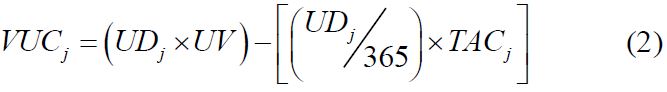
j = Year of service in question
VUCj = Annual vehicle unavailability cost for year j
UDj = Unserviceable duration in days per service year j
UV = Utilization value in USD/day
TACj = Total annual cost in USD per service year j
There is one unique value of UV for every vehicles group class (constant), decided by management, to represent the value of the opportunity cost of not utilizing that vehicle due to unavailability. Eq.(2) is used to compute the unavailability costs for both the defender (VUCj) and the challenger (VUCk). For the defender, historical data during passed years of service will be used to find unserviceable duration through its remaining service life by means of forecasting. However, to determine the challenger’s unavailability cost for year (k), the defender’s working in service group class vehicles sample historical data will be used.
3.4 VEHICLE PRIORITY FACTOR
Management should decide the real weight for the additional cost aside from the original economic weight, and to what limit the unavailability of certain vehicle may affect its utilization as useful and productive. Vehicle Priority Factor (VPF) is a percentage determined by management to represent priority level of the vehicle, i.e. the importance to keep it available, operational, and serviceable. This factor can play main role in performing the heuristic in case of adding the unavailability measure. Based on the unavailability effect, the new annual expenses will be the original annual expenses plus VUC multiplied by VPF value for a certain vehicle class, that is:

Both total marginal costs (TMCj) for the defender during its remaining anticipated service life, and the challenger’s EUACch will be applied only in case of new values for TAC.
3.5 DEFENDER AND CHALLENGER COST PROFILES
Calculation of the total cost for any year (j), or total cost for an additional year of service during lifecycle of a vehicle is called total marginal cost (TMC j (i%)), which is equal to:

MVj = Market value of the vehicle at the end of service year j.
TACj = total annual costs (new) of vehicle during service year j.
EUAC of available replacement vehicle is an important tool in implementing the heuristic. EUACch represents the perspective of cost of same class future vehicle at which can be estimated based on the challenger cash flow profile. EUAC through service year (k) can be calculated as follows:
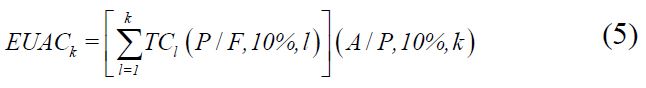
where, TMCl is the total marginal cost for year l.
3.6 SELECTION OF ALTERNATIVE STRATEGIES
The aim here is to find the set of alternative strategies preferable to the existing strategy of the keeping the defender (do nothing). The economic decision criterion starts by defining the suggested vehicle replacement strategies (Aj), where (j = 1) to (n + 1), which are followed throughout the study period (n). If a cost associated with following strategy (j) is smaller than a cost of following do nothing alternative, i.e. (An+1), then strategy (j) is said to have the advantage of a lower cost over strategy (n+1). Finding a set of alternative strategies preferable to (n+1) represents the future worth cost advantage of strategy j(FWCAj), which is calculated as follows:
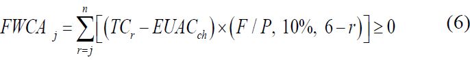
where,
FWCAj = future worth cost advantage of strategy j over strategy (n + 1)
TMCr = total marginal cost of Defender during year r
EUACch = equivalent uniform annual cost of challengerIf the total marginal cost of the defender at (j) exceeds the EUACch, then FWCAj is evaluated. The year (j) at which FWCAj is the maximum value strategy (Aj) is the best strategy, in addition to other acceptable strategies when FWCAj is positive.
4. THE HEURISTIC
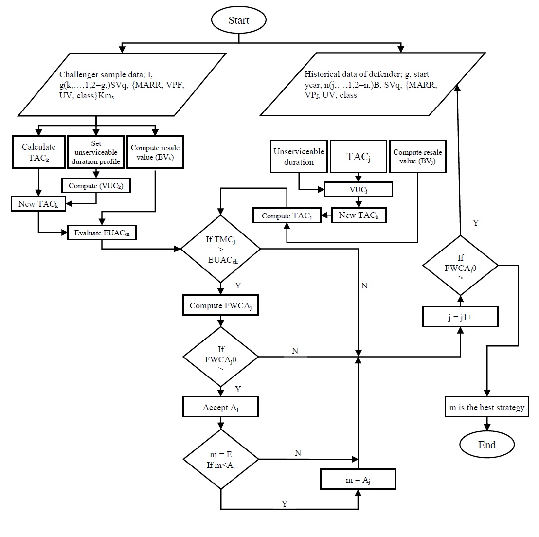
Fig.1. Flow diagram for the developed heuristic
Based on the previous analysis, the proposed heuristic for existing operational vehicle replacement is developed. It can aid in choosing strategies of replacement by implementing the analysis discussed earlier. Following are the steps:
- 1. Start with an existing vehicle in service and obtain input data for the challenger and the defender. Historical data of the defender and the challenger’s sample data. 2. Based on the challenger’s input data and using Eq.(1), calculate TACk according to prospective traveled distance for the challenger and TAC equations resulting from sample data of the defender class vehicles.
- 3. Evaluate the unserviceable duration for the challenger during its anticipated years of service according to its sample data, and compute the challenger resale values BVk by using DBD method. 4. Using DBD method to estimate the defender resale values BVj. Develop defender’s unserviceable duration and TACj during (j) from year (1 to n) by using forecasting techniques.
- 5. Compute VUCk and VUCj using Eq.(2).
- 6. Apply Eq.(3) to estimate new TACk and TACj by substituting the resulted values in step (5) and values of original TACk and TACj.
- 7. Based on the Challenger cash flow profile resulting from steps (6) and (3), Evaluate EUACch using Eq.(5).
- 8. Compute TMCj of the Defender according to its cash flow profile resulted from steps (6) and (4) based on Eq.(4).
- 9. In the decision-making process, compare TMCj with EUACch.
- 10. Find year j during which TMCj exceeds the EUACch.
- 11. Calculate the FWCAj of strategy j over An+1 using Eq.(6) evaluated at the end of the study period.
- 12. If the FWCAj of strategy j is nonnegative, then strategy j is acceptable. Otherwise, strategy j is rejected.
- 13. If there is more than one acceptable strategy, then a strategy with the highest cost advantage is identified as the best strategy.
The Fig.1 illustrates and summarizes the above heuristic.
5. CASE STUDY
To demonstrate the developed heuristic, a case study for the Royal Air Force (RAF) fleet of vehicles is presented from Jordan. RAF owns several classes of vehicles operating in service. They are distributed in different areas inside Jordan’s air bases, units, airports, the head quarter, and other places, see Fig.2. These vehicles, equipment, and maintenance program is the responsibility of and performed by RAF [23].
Existing vehicles in service are classified according to several criteria such as: vehicle type and model, vehicle purpose and usage, vehicle capacity, vehicle payload, vehicle utilization, engine capacity, vehicle wheel drive system, and other criteria decided by management. Any vehicle that is contained in the defender group class can be treated as a replacement vehicle to the existing vehicle or as challenger. Table.1 illustrates the developed classification of the general use vehicles in RAF fleet.
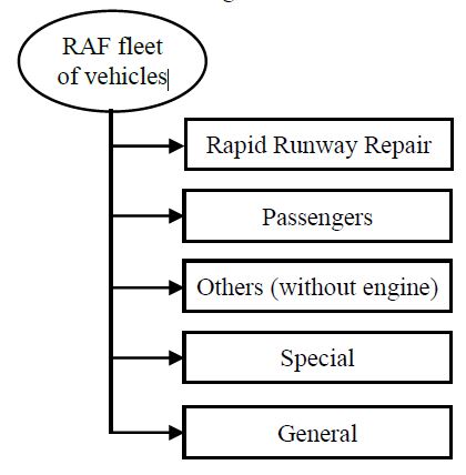
Fig.2. Main types of vehicles in RAF fleet
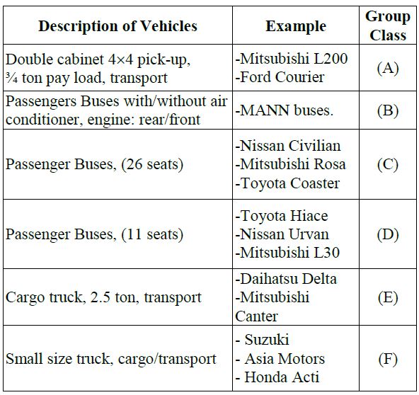
Table.1. Classification of general use vehicles in RAF fleet.
RAF has an equipment maintenance system (EMS), which is software used to control and develop the work process (human and equipment). It is applied to all electrical and mechanical equipment including vehicles except aircrafts. EMS is used to assist in registering historical data records of equipment, based on work-shop process, year of service, maintenance and repair cost, fixed and other variable cost, unserviceable duration during its maintenance in the workshops, and man working hours during the equipment service life. These data will be used in the case study. The vehicle under study is assumed to be vehicle (x) included in group class (A).
5.1 REQUIRED INPUT DATA
The following input data for the challenger and the defender based on RAF’s files and EMS are used in the case study. For the defender;
- 1. Age of vehicle (x) = 7 years.
- 2. Starting service year is 1993.
- 3. Group class (A).
- 4. Anticipated remaining service life (n) = 6 years.
- 5. Present resale value = 4000 USD.
- 6. Salvage value = 1850 USD.
- 7. MARR = 10%.
- 8. Historical cost data for years in service1993 to 1999 were equal to 734, 719, 836, 769, 887, 981 and 1238 USD respectively.
- 9. Historical data of unserviceable duration for years in service 1993 to 1999. The unserviceable duration for vehicle (x) during the past years of service was 2, 6, 6, 13, 7, 37, and 9 days respectively.
- 10. Utilization value (UV) for vehicle (x) = 23 USD/day
Input data for the challenger:
- 1. Initial capital investment = 8500 USD.
- 2. Salvage value = 1850 USD.
- 3. Anticipated service life = 13 years, k = 1,2 …13.
- 4. Data for class (A), for 35 vehicles TAC with respect to distance traveled during years of service 1, 2…13.
- 5. Data for class (A) for 35 vehicles unserviceable duration against years of service 1, 2…13.
- 6. Prospective traveled distances for years of service 1, 2…13 = 50,000 km/year.
Vehicle priority factor (VPF) for the A, B, C, D, E, and F vehicle classes of Table.1 are 0.25, 0.55, 0.30, 0.25, 0.50 and 0.20 respectively according to maintenance and repair work priority criteria used in the RAF main workshop.
6. ANALYSIS AND DISCUSSION
Using the input data, the Vehicle (x) TACj and BVj values are shown in Table.2. The Eq.(1) was used to determine TACk for the challenger, Table.3. Hence, forecasted unserviceable duration and VUCj are shown in Table.4 using Eq.(2). The unserviceable duration of the challenger (UDk) during its 13 years of service was parameterized and the challenger VUCk estimated, Table.5. Next, new costs for both the vehicle (x) and its challenger are calculated, according to unavailability costs in addition to the effect of VPF as per Eq.(3). The existing vehicle (x) and it’s the challenger cash flow profiles are summarized in Table.6 and Table.7. Table.8 shows the TMCj for vehicle (x) during service year j based upon Table.6 and Eq.(4). Also, based on Table.7 and Eq.(5) the EUACch was determined to be 2342 USD with eight years economic life.
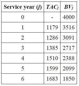
Table.2. Vehicle (x) TACj and BVj during its remaining anticipated service life
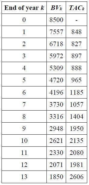
Table.3. Challenger’s resale values and TACk during its anticipated service life
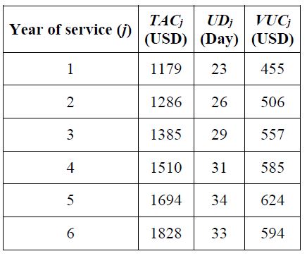
Table.4. VUCj of vehicle (x) during its remaining anticipated service life
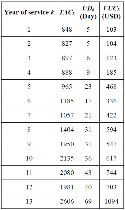
Table.5. Challenger’s VUCk during its anticipated service life
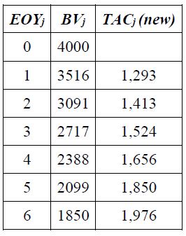
Table.6. Vehicle (x) cash flow profile
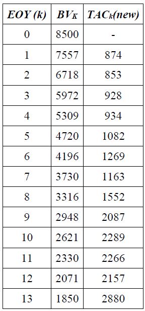
Table.7. Challenger’s cash flow profile
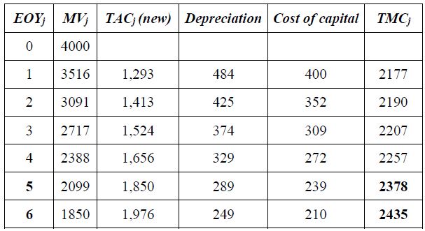
Table.8. TMCj for the vehicle (x) during the study period
The proposed strategies of replacing vehicle (x) during the study period n = 6 years, are A1 through A7. For strategy A1 the challenger is introduced at the beginning of year one, strategy A2 the challenger is introduced at the beginning of year two and so on, while strategy A7 represents the null. Vehicle replacement cannot be treated in isolation and solved by rules and formulas. Any existing vehicle in service has its own operational condition, environment, driving habits, utilization fluctuations, repair and maintenance events, and other considerations. The developed heuristic can make the decision making accurate and include more variables. However, accurate historical data of costs, unserviceable duration, and other parameters are required since they are the basis of estimation of cost profiles. Also, the forecasting techniques and depreciation method used in the analysis may affect model results, since vehicles are variable in their performances, usage rates, and other operating conditions, more research is needed. Comparing the EUACch and TMCj shows that TMCj > EUACch for years 5 and 6, and the FWCA for A5 and A6 are 133 and 93 USD respectively.
Hence, both strategies A5 and A6 can be accepted. However, A5 is the best strategy to replace vehicle (x), since FWCA5 is the highest. The challenger can be introduced at the beginning of year 5. Replacement might be postponed for one year with payoff of at least 40 USD. The difference in costs continues to grow, and replacement becomes more urgent with the passage of time. The economic analysis is time dependent, the current decision taken by management to replace or postpone the replacement of a certain vehicle now might change according to new inputs; technological changes and the availability of new better replacement vehicles. Also, economic impact of a replacement decision is dependent on the study period for the analysis.
7. CONCLUSIONS
This study presented a scheme to deal with the replacement strategies for existing operational vehicles. The developed heuristic evaluates vehicle replacement policy from the management point of view, taking into consideration the effect of depreciation, maintenance, recurring cost, utilization value, availability and serviceability. The developed heuristic can provide management with a decision making tool for replacement and to assist in developing maintenance policy, which aims at improving vehicle’s availability and reducing costs. It can aid decision-makers with long-term planning and the procurements of vehicles and parts. The implementation of the heuristic in an organization requires integrated education, training and practicing throughout all maintenance sectors and vehicles management, in order to increase useful effective time and reduce waste during maintenance events. The developed heuristic was applied to RAF vehicles’ fleet and proved to be a valuable in defining and evaluating available alternatives and in conducting trade-off analysis.
REFERENCES
[1] John A. White, Kellie S. Grasman, Kim Lascola Needy and David B. Pratt, “Fundamentals of Engineering Economic Analysis”, John Wiley and Sons, 2013.
[2] Robert E. Stewart, “A Practical Computer System to Assist with Equipment Replacement Decisions”, Proceedings of Spring Annual Conference, pp. 287-305, 1980.
[3] Rommert Dekker, “Applications of Maintenance Optimization Models: a Review and Analysis”, Reliability Engineering and System Safety, Vol. 51, No. 3, pp. 229-240, 1996.
[4] William G. Sullivan, Elin M. Wicks and C. Patrick Koelling, “Engineering Economy”, 16th Edition, Pearson, 2014.
[5] W. Grant Ireson, Clyde F. Coombs and Richard Y. Moss, “Handbook of Reliability Engineering and Management”, 2nd Edition, McGraw-Hill Professional, 1996.
[6] Donald G. Newnan, Ted G. Eschenbach and Jerome P. Lavelle, “Engineering Economic Analysis”, 12th Edition, Oxford University Press, 2013.
[7] R.W. Drinkwater and N.A.J. Hastings, “An Economic Replacement Model”, Journal of the Operational Research Society, Vol. 18, No. 2, pp. 121-138, 1967.
[8] Gerald L. Thompson, “Optimal Maintenance Policy and Sale Date of a Machine”, Management Science, Vol. 19, No. 9, pp. 543-550, 1968.
[9] R.N. Wadhawan and F.G. Miller, “Forecasting Fleet Vehicle Replacement in a Dynamic Situation”, Maintenance Management International, Vol. 6, pp. 215-222, 1986.
[10] Hiroshi Matsuo, “A Modified Approach to the Replacement of an Existing Asset”, The Engineering Economist, Vol. 33, No. 2, pp. 109-120, 1988.
[11] C.E. Love and R. Guo, “Utilizing Weibull Failure Rates in Repair Limit Analysis for Equipment Replacement/ Preventive Maintenance Decisions”, Journal of the Operational Research Society, Vol. 47, No. 11, pp. 1366-1376, 1996.
[12] Alfonso J. Pedraza‐Martinez and Luk N. Van Wassenhove, “Vehicle Replacement in the International Committee of the Red Cross”, Production and Operations Management, Vol. 22, No.2, pp. 365-376, 2013.
[13] Cho Sungjin and John Rust, “Is Econometrics Useful for Private Policy Making? A Case Study of Replacement Policy at an Auto Rental Company”, Journal of Econometrics, Vol. 145, No. 1, pp. 243-257, 2008.
[14] Dennis C. Dietz and Paul A. Katz, “U.S West Implements a Cogent Analytical Model for Optimal Vehicle Replacement”, Interfaces, Vol. 31, No. 5, pp. 65-73, 2001.
[15] Yoshinori Suzuki and Gregory R. Pautsch, “A Vehicle Replacement Policy for Motor Carriers in an Unsteady Economy”, Transportation Research Part A: Policy and Practice, Vol. 39, No. 5, pp. 463-480, 2005.
[16] Konstantinos J. Liapis and Dimitrios D. Kantianis, “Depreciation Methods and Life-cycle Costing (LCC) Methodology”, Procedia Economics and Finance, Vol. 19, pp. 314-324, 2015.
[17] B. Dhillon, “Life Cycle Costing: Techniques, Models and Applications”, Routledge, 2013.
[18] David V. Spitzley, Darby E. Grande, Gregory A. Keoleian and Hyung Chul Kim, “Life Cycle Optimization of Ownership Costs and Emissions Reduction in US Vehicle Retirement Decisions”, Transportation Research Part D: Transport and Environment, Vol. 10, No. 2, pp. 161-175, 2005.
[19] John A. White, Kenneth E. Case and David B. Pratt, “Principles of Engineering Economy Analysis”, 4th Edition, John Wiley and Sons, 1998.
[20] Andrew Chesher, Robert Harrison and Joffre D. Swait, “Vehicle Depreciation and Interest Costs: some Evidence from Brazil”, Transport Research for Social and Economic Progress, Vol. 3, pp. 2137-2157, 1981.
[21] U.S. Department of Transportation, “Cost of Owning and Operating Automobiles, Vans and Trucks”, Intellichoice, 1991.
[22] John Alico, “Appraising Machinery and Equipment”, McGraw-Hill, 1988.
[23] Royal Air Force Directorate of Maintenance, “Equipment Maintenance System”, 1999.